Formation of New Connections by a Generalisation of Hebbian Learning

Kingsley J. A. Cox and Paul R. Adams

Department of Neurobiology and Behavior, SUNY Stony Brook, NY 11794, USA

Correspondence should be addressed to P.R.A. (padams@notes.sunysb.edu),

Phone 516 632 6938 Fax 516 632 6661

 

 

Abstract

Recent experiments suggest that activity-dependent synaptic strengthening occurs in a digital but anatomically imprecise fashion. We model this process computationally and mathematically and show that the resulting smearing of neural connections depends on the error rate for synapse placement and on the spatial sharpness of neural correlations. We argue that while such errors lower the current efficiency of neural networks, they are useful for flexible learning. One way to limit such wiring errors is to compartmentalise the molecules that trigger strengthening, in spines. However, such direct error reduction strategies hinder brain miniaturisation. The brain may therefore also use an indirect strategy, restricting plasticity to highly-correlated neurons.

 

 

1. Introduction

Much theoretical work suggests that neural networks can self-organise to perform useful tasks if the connection strengths are set by activity-dependent, Hebbian, mechanisms [2,4, 21]. Because real neurons are connected by costly and voluminous axons, it seems unlikely that all possible connections are permanently wired so that their strengths can be immediately and continuously updated by Hebbian learning. It is more plausible that only a subset of the possible connections are wired at any particular time, and that Hebbian mechanisms are supplemented by local sprouting [3,12]. However only a few authors [13,23,30] have explicitly considered such supplementary rules, usually in the context of specific models of particular neural functions. We report here a simulation and analysis of a generalisation of a Hebbian rule which allows for local, activity-dependent formation of new connections [1].

Our model is supported by two recent findings about synaptic strengthening in hippocampal CA1 neurons. First, if a CA1 neuron's activity is paired with that of a presynaptic CA3 neuron, then synaptic strengthening occurs not only between the co-active pair, but also between one member of the pair and nearby pre- or postsynaptic neurons [7,14,26]. This is sometimes referred to as "volume learning" [22], and may reflect spillover of transmitters or second messengers beyond the co-active synapses. Second, in cases where the co-active pair is connected by what appears to be a single synapse, strengthening occurs in an all-or-none, stochastic fashion [24]. Thus the strengthening of individual synapses resembles a process of synaptic replication, since one functional synapse gives rise, after a random delay whose mean value depends on the intensity of the co-activity, to two functional synapses. It has been suggested that functional doubling is then followed by structural doubling [9,6,29], though this is controversial [28].

In our model new synapses created by correlated firing of a pair of neurons are not always perfectly placed at the connection linking the correlated neurons. Such errors in the placement of new synapses lower the precision with which networks can be wired, but they also allow exploration of new connectivity patterns. Both the harmful and beneficial effects of such "heterosynaptic" plasticity errors depend on the profile of correlations across the network, and it is suggested that an optimal balance could be achieved by appropriate measurement of such profiles.

 

2. The Model

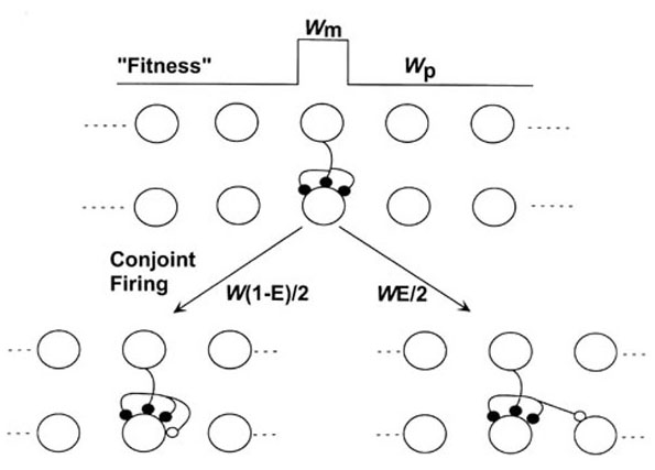
Figure 1

Fig 1. A model for the formation of new synaptic connections. A layer of presynaptic cells can connect to a layer of postsynaptic cells, but only the connections (and possible connections) formed by one of these cells are considered. In the top part, an existing connection, composed of 3 synapses (solid) , is shown. As a result of correlated or synchronous firing, an additional synapse is created. This new synapse (open circle) can appear either on the postsynaptic component of the connection (shown bottom left) or on a neighbor of that postsynaptic cell (left or right, but only the latter shown here). Both the creation of new synapses and their misplacement occur stochastically, the former with probability w, and the latter with probability E. The former but not the latter vary across the array. The erroneous placement of new synapses is a form of heterosynaptic error and is analogous to point mutation in DNA. The paper discusses the simple case where fitness of one possible connection (w_m) is higher than that of surrounding possible connections (w_p; see fitness profile sketched at the top of the figure).

 

The model is summarised in Fig 1. A single presynaptic neuron can make connections to any of a row of N postsynaptic neurons. The connection to the ith postsynaptic neuron is composed of y_i synapses, where y_i can range from 0 (meaning that the connection is absent) to M, the total number of synapses formed by the presynaptic neuron, which is held constant (by divisive renormalisation). We assume that the strength of each connection, y_i, depends on the past history of pre- and post-synaptic activity at that connection, in a Hebbian manner. In the simplest case, if V_pre is the activity of the presynaptic neuron, and V_i of a postsynaptic neuron,

dy_i/dt = k_iV_preV_i

where k_i is a (possibly connection-specific) learning constant. If learning occurs continuously, then as the connection strengthens, the postsynaptic firing rate will gradually increase. In the simplest case, if g_i is a (possibly connection-specific) synapse effectiveness,

V_i = g_i y_i V_pre

Writing w_i = k_i g_i V ²_pre we have

dy_i/dt = w_i y_i..................................................(1)

We refer to w_i as the "fitness" of a connection. Biophysically it is related to the degree of "correlation" between the pre- and post-synaptic neuron. Eq 1 is intended to capture the autocatalytic nature of many models of connection formation. As discussed by von der Malsburg and Willshaw [18], together with competition it leads to the elimination of all but the most highly-correlated connections. The idea of the fitness of a connection is a convenient simplification of the actual rates of growth, which in unsupervised learning models are set by statistical features of the input ensemble. Thus in deriving equation 1 we implicitly assume that the rate of growth depends on a temporal average of V_pre², and we neglect contributions from other inputs to neuron i. In general these contributions will tend to make growth less autocatalytic, which will tend to increase the spread of synapses (see Section 4). Thus the simplifications in our model tend to weaken, rather than strengthen, our conclusions.

We could instead obtain Eq 1 by assuming that correlated firing actually causes a functional doubling of individual synapses, as implied by the results of Petersen et al [24]. In that study, it was found that after the initial doubling the connection was refractory to further pairing. However, other work suggests that such refractoriness gradually disappears as a result of protein synthesis [15], possibly culminating in the formation of a structurally new synapse [6]. Interestingly, the removal of refractoriness appears to require the presence of dopamine [15], suggesting a simple mechanism for reward-based learning. The new synapse would presumably eventually respond to further pairing in the same way as the original synapse, by stochastic functional doubling. However, the existence of refractoriness has so far precluded a quantitative investigation of the rules of synaptic strengthening. It is possible that repeated pairing, sufficiently widely spaced, would lead to an exponential growth in synaptic strength (in the absence of normalisation), as implied by the use of fitnesses. However, it is also possible that each identical pairing adds just one synaptic unit (the conventional linear Hebbian growth model). In the latter case, fitnesses would have to be introduced indirectly, by considering the autocatalytic nature of cell firing and Hebbian strengthening (as in the above derivation of eq 1). Von der Malsburg and Willshaw [18] have previously noted the attractions of the simple fitness view, in which Eq 1 is literally true, and w reflects the correlation between the pre- and post-synaptic cells. However, they also point out that combined with the autocatalytic effect of neuron firing the replication rule can lead to hyperbolic growth and lock-in of chance initial configurations. This problem could be avoided by offline conditional renormalisation of synaptic strengths.

If the connections are composed of discrete synapses, and if Hebbian strengthening is a stochastic all-or-none process [24], then w_i represents the probability that in a small time interval a synapse will "replicate" as a result of correlated activity across the connection to which it belongs. If the replication process is perfect, then the new synapse will appear at that connection. However, we assume that the new synapse is assigned to that connection only with probability (1-E), and that it can instead appear at either of the neighboring connections onto cells i-1 and i+1 (which may or may not already exist) with probability E/2. Although a synapse appears at a connection, which has a fitness w_i, it is sometimes convenient to speak of it appearing at a neuron, and to refer to the fitness of that neuron (since it is awkward to speak of non-existent connections). E is the error rate for the formation of new synapses. Errors in the placement of new synapses could result from a combination of molecular noise in the signal cascades that underlie strengthening, and spread of messenger molecules beyond the synapse across which correlated activity occurs. Volume learning experiments [7,14,26] suggest that such errors may occur, although they have not been previously interpreted as such, and do not provide direct evidence for the formation of new connections. Other work [3,8,12] suggests that new connections form in the vicinity of existing connections, by a sprouting process, but has not determined the causes.

 

3 Simulations

We simulated 2 versions of the model. In the first version, the "imposed fitness model", fixed w_i values at each connection were used to calculate the probabilities that in each time step an existing synapse would replicate. If a synapse replicated, then the new synapse was placed at the parent connection with probability (1-E), or, with probability E at either of the 2 neighbours (the choice made with equal probability). These 3 stochastic processes, "replication", "mutation" and "choice", were implemented using random numbers uniformly distributed between 0 and 1. After updating all the synapses at each connection (an "epoch"), the total number of synapses M_e was compared to the fixed number M (either 1300 or 13,000, see figure legends). The number of synapses at each connection was then multiplied by M/M_e, to return the total strength to M (divisive renormalisation). This renormalisation was done deterministically. These steps were repeated until the connection strengths reached stable values.

We studied the particularly simple, but instructive, case, where all the connections except one had the same low level of fitness, w_p. The remaining connection had a higher level of fitness, w_m. This fitness profile corresponds to a single sharp mesa of strong correlation (perhaps imposed by an input pattern) in a surrounding plateau of weaker correlations (due for example to spontaneous firing of neurons). In most of the simulations the high fitness connection was placed on the leftmost neuron of the postsynaptic row. This version of the model has only 3 parameters, E, w_m, w_p, together with an initial profile of synapses. Reflection at boundaries was assumed.

In the second version, the "reward-based model", the fitnesses were calculated, not imposed. The postsynaptic neurons responded linearly to synaptic input from the presynaptic neuron, with an output which was then compared with the desired, or target, output. The strength of each connection was then stochastically updated according to Eq 1. However, w_i was now not imposed but calculated as the product of a global reward/penalty term and a local "change in coincidence" term. The global reward/penalty term was the epoch-to-epoch change in the root mean square difference between the current outputs of each neuron and their desired outputs. The local coincidence change was proportional to the difference of the current and previous outputs. Each synapse was subject to stochastic and possibly erroneous replication as in the imposed model. Because in this model w can be negative, synapses could also stochastically die. Total synapse number M_e was renormalised at the end of each epoch. This model has only 1 parameter (E), together with choices of target and an initial profile of weights.

 

3.1 Steady State Properties of the Imposed Fitness Model

Whatever the starting profile the final distribution of synapses depended only on E and w_m/w_p (with some superimposed fluctuations due to the random nature of synapse birth and placement). Fig. 2a shows the steady state distribution of synapses achieved with various error rates and a fixed fitness profile. As the error rate increases, synapses spread increasingly beyond the fittest neuron. These steady state distributions arise in the following manner. In the mesa region, on the leftmost neuron, synapses are being formed at a rate which is higher than average. However, there is an error efflux of synapses from the fittest connection to the adjacent connection, and thence to further cells. In the steady state this error efflux is exactly equal to the local excess production of synapses, so that the strength of the fittest connection is constant. In the plateau region, synapses are being produced at a below average rate, but again this underproduction of synapses is exactly balanced by the error influx from the fitter connection.

Increasing the fitness ratio w_m/w_p at a fixed error rate had the opposite effect, focussing the synapses on the fitter neuron (Fig 2b). Thus the effects of error and relative fitness are opposed. Precise connections can be achieved either by lowering error rates or increasing fitness ratios (that is, increasing the sharpness of neural correlations). In the limit of zero error rates, implicitly assumed in conventional Hebbian models, or of completely specific correlations, connections could be made perfectly.

Figure 2

Fig 2. Steady state connection strength profiles for various error rates (left) or fitnesses (right). In each case the left neuron was the fittest, and there were 13 neurons and 1300 synapses. The average number of synapses on each neuron achieved at equilibrium is shown for various values of error rate E and fitness ratio w_m/w_p. As error rates increase (left graph) or fitness ratios decrease (right graph) synapses become more spread out. Values of E used in part a were 0.1 (circles), 0.2 (squares), 0.3 (inverted triangles) and 0.4 (triangles), with w_m/w_p = 1.4 throughout. Values of w_m/w_p used in part b were 1.11 (circles), 1,.25 (squares), 1.42 (inverted triangles), 1.66 (triangles), with E = 0.2 throughout.

Analysis of our model (see Section 4 Eq 8) suggests that if there are enough synapses and postsynaptic neurons the decay of connection strength beyond the fitter neuron should be exponential. This appeared to be the case (Fig 3a). The accuracy of connections can thus be defined by a length constant 8, which depends on E and w_m/w_p. Fig 3b shows how 8 varied with the error rate and the fitness ratio, confirming their reciprocal influence. Our analysis (Section 4 Eq 10) suggests that relation shown in Fig 3b should be linear, with a slope of 2. The data points fitted a straight line with a slope of 2.2 quite well. The parameter 8 essentially measures over how many neurons connections are smeared by the combined influence of error and patterned neural activity.

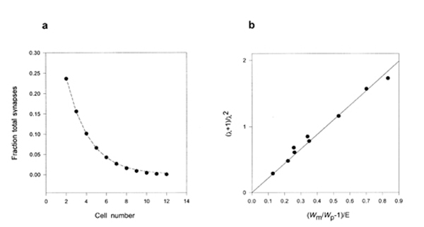
Figure 3

Fig 3. Part a shows the fraction of the total number of synapses (13,000) that form at less fit connections (i.e. the plateau region) compared to an exponential curve of length constant 8 = 2.45 neurons). E = 0.2; w_m/w_p = 1.05. Cell 13 received no synapses and was omitted. Part b shows the reciprocal effects of relative fitness and error rate. Each point was obtained for a different combination of w_m/w_p and E from data like that shown in part a. The linear regression through the origin has a slope of 2.2, compared to the predicted slope 2.0 (see Methods Eq.10).

 

3.2 Kinetic Properties of the Imposed Fitness Model

What happens if connections are equilibrated at one fitness profile, which is then suddenly changed? There are 2 possibilities. The initial equilibrated connections might already include the newly fittest connection, which will immediately start growing in strength. However, if the newly fittest connection is rather far away from the originally fittest connection, for example several length constants away, it might not be initially available, especially if there are limited numbers of synapses (small M). In this case there will be a lag period before synapse turnover and placement errors in the less fit region lead to accidental formation of the correct connection. Once formed, the preferred connection will then rapidly strengthen.

Our simulations confirmed both of these expectations. Fig 4 shows the redistribution of synapses that occurs when the fittest connection shifts drastically, from the leftmost neuron to the rightmost neuron. The initial rather broad distribution of synapses corresponded to the steady state achieved with E = 0.05 and w_m/w_p = 1.05. After the switch the few synapses already on the rightmost neuron flourish, pushing down the numbers on the previously fitter neuron. Connections near the center of the row only slightly adjust their strength.

Figure 4

Fig 4. Migration of synapses following a mirror reversal of fitness. Initially synapses were equilibrated with the leftmost connection ( on cell 1) being 5% fitter than the others. This resulted in the zero epoch profile. The rightmost connection (on cell 13) was then made 5% fitter than the others, and the resulting profiles plotted for successive epochs (after binning results for 20 consecutive epochs to reduce noise). M = 13,000; E = 0.25.

Fig 5 shows the establishment of synapses on the fitter, rightmost, neuron, when initially all the synapses were located on the leftmost neuron. There is a waiting period while synapses diffuse away from the initial focus. As soon as the first synapse reaches the rightmost neuron, the connection flourishes. Because synapse creation is stochastic, this waiting period varied randomly with different runs of the same simulation. The waiting period became shorter as the total number of available synapses M was increased.

Figure 5

Fig. 5. Kinetics of appearance of synapses at the fittest connection, on the rightmost neuron (cell 13). All synapses were initially placed on the leftmost neuron. The number of synapses on the right neuron was plotted at successive epochs. The total numbers of synapses M were 26,000 (left 5 runs), 13,000 (middle 5 runs) or 6,500 (right 5 runs). Note that there is a variable delay before the formation of the first synapse on the fittest neuron, followed by rapid increase in the connection strength. However, because for the parameter values used (E = 0.1, w_m/w_p = 1.05) the length constant is quite high, the fittest neuron only gains about half of the total number of synapses.

 

3.3 A Slightly More Realistic Model

The above model is rather abstract, since it lumps all the specific patterns of neural activity that underlie real information processing into a single parameter, "fitness", that describes how fast a connection is growing. We also simulated a slightly more realistic situation, in which the "fitnesses" were not externally imposed, but emerged as a result of reward-based learning. This modified model was loosely based on previous work [20] in which a Hebbian learning rule incorporated a reward/penalty term. In that model neural firing occurred stochastically in response to synaptic input. If the actual output firing pattern moved closer to the desired output pattern, a reward signal was generated which multiplicatively increased Hebbian strengthening. In our modification, in keeping with the spirit of our approach, the stochastic property that caused fluctuations in output was formation of synapses. At connections where synaptic turnover and/or error caused increases in strength which were temporally associated with improvements of performance, further increases in strength were made. If improvements in performance were coupled in decreases in strength of connections, further decreases in strength were made. Thus the sign and size of learning at a connection depended on a global assessement of performance (a reward or penalty) as well as a local, stochastic change in synaptic strength (decrease or increase).

Once again the aim was simply to create a strong connection onto a designated, target, neuron, this time by applying rewards whenever the output fluctuated toward the target, and penalties when it fluctuated away. Even though the "teacher" is perfect (always applying appropriate global rewards or penalties), there exists the possibility that some connections fluctuate in strength in the "wrong" direction and are rewarded because other connections fluctuated in the "right" direction and generated a net improvement. This "masking" effect is the Achilles heel of simple reward models, and it means that inappropriate connections exhibit finite fitnesses, which together with errors in the placement of synapses result in smearing. Fig 6 shows examples of these simulations, in which the central neuron in an array of 13 was designated as the target. Once again as the error rate increased the connection spread progressively beyond the target. We also found that, at least in small arrays, reward-based learning could cause connections to shift appropriately from the leftmost to the rightmost neuron (not illustrated).

Figure 6

Fig 6. Steady-state profile of synapses attained in a reward-based model. The central neuron (cell 7) was designated as the target for all 1400 synapses. Epoch-to-epoch fluctuations in the numbers of synapses at each connection, caused by stochastic replication and mutation, led to variations in the locations of these synapses. These locations, compared to the target locations, determined a global "reward" or "penalty" which, together with the sign and size of local fluctuations in synapse number, set the per epoch probability that a synapse replicates or dies (see Methods). The following error rates were used : 0.1 (circles); 0.2 (squares), 0.3 (triangles); 0.4 (inverted triangles).

 

4. Analysis.

The imposed fitness model can be analysed under some simplifying assumptions.

Discrete positions (different i values) are replaced by a continuous distance parameter x. The continuous density of synapses at a connection is y(x,t), though in the following dependencies on x and t are not explicitly written. Because we assume that the total number of synapses made by the presynaptic neuron is constant, we modify Eq 1 [18] to

dy/dt = (w - <w>) y ............................................(2)

where <w> is the average fitness of a connection defined by

<w> = ò w.y dx / ò y dx........................................(3)

Equations (2) and (3) represent the redistribution of synapses that occurs as a result of error-free correlation-induced replication followed by divisive renormalisation. No assumption is made as to the physiological mechanism of such renormalisation, which merely enforces competition between different connections. The second process contributing to redistribution is error. Since error occurs randomly to the left or right, it can be represented as a diffusion process:-

¶y/ ¶t = 0.5 wE ¶ ²y/ ¶x^{2 .................................................}(4)

Combining Eqns 2 and 4 we have

¶y/ ¶t = (w -<w>) y + 0.5wE ¶ ²y/ ¶x²................(5)

The first term on the right describes the growth (decay) of fitter than average (less fit than average) connections, while the second term describes the random left/right placement of new synapses. Equation 5 is nonlinear (because by equation 3 <w> depends on y), but in the steady state y has a fixed profile and <w> is a constant, and (5) reduces to an linear second order ordinary differential equation :-

d²y/dx² = 2(<w> - w)y/ wE................................(6)

In the simulations w = w_m over some small central fraction of the total length of the array L, and w = w_p over the rest of the array (w_m > w_p). In the high fitness region w_m exceeds <w> and

y_m = A sin x/ l _m + B cos x/ l _m..........................(7)

while outside the mesa w_p is less than <w> and thus

l _p = C exp -x/ l _p + D exp x/ l _p.......................(8)

where

l _m² = E w_m /2 (<w> - w_m) and l _p² = E w_p /2 (<w> - w_p) ....................(9)

l _p is a length constant describing the decay of synapses beyond the high fitness region. If l _p << L (like an infinite cable), then there will be no synapses at x = L, and thus D must be zero. An approximate expression for l _p can be derived from equations (3) and (8):

(2 l +n)/ n l ² = 2(w_m/w_p - 1)/E ......................(10)

where n is the number of neurons in the high fitness zone, provided n is small compared to l _m. Equation 10 shows the reciprocal influence of w_m/w_p and E. Note that in our simulations the single high fitness neuron was located at the end of the row. Because of reflection at the boundary this is equivalent to n = 2, giving the expressions plotted in Fig 2b.

If sprouts occur not as the result of heterosynaptic strengthening errors ("mutations"), but at some activity-independent basal rate S, the term wE in equation (5) should be changed to S. The spread of synapses will now depend on the difference, not the ratio, of the mesa and plateau fitnesses, each relative to S.

 

5. Discussion

The models we simulated and analysed are very simple but the issues at stake are important and little discussed. We find that if correlations are not extremely sharply peaked and if new synapses are not precisely placed, then connections become smeared out. In general this smearing would be expected to lower the performance of a neural network compared to one in which connections are perfectly specified by conventional, error-free, Hebbian mechanisms. However, this smearing also has advantages. First, existing superfluous connections formed by error and retained because of significant background correlations are seeds for future learning. In essence such superfluous connections are already implicit in conventional, fully-connected, Hebbian models, since neuron pairs linked by negligible synaptic weights remain connected and able to promptly adjust their weights should the activity to which they are exposed change. Second, if connections are plastic, they will turn over when exposed to neural activity, and thus, by our hypothesis, generate novel connections, which allow new network configurations to be tested. However, this will be a slow process (see Fig 4), especially if individual synapses are strong (relative to the firing threshold), and connections are therefore sparse. If synaptic noise is important for reward-based learning, then individual synapses will also have to be relatively strong.

A more conventional approach to the neural wiring problem is to assume that connections are initially formed promiscuously, and eliminated by competition. The difficulty that these abundant initial connections will occupy inordinate space is partly shoved under the carpet, since the final connections can be very sparse. However, there is considerable plasticity in the adult brain [8], including sprouting [12], and it is quite possible that adult learning is not restricted to the adjustment of existing connections. We postulate that even in adults new connections are continuously formed in a selective manner: they are only formed when synaptic strengthening occurs, and they only form in the vicinity of existing connections. These postulates seems reasonable. However, it is possible that instead new connections are formed continuously in the absence of neural activity, and then are pruned back as a result of ongoing anti-Hebbian learning. This alternate model would have similar properties to the one we explored (see Section 4).

 

5.1 Comparison to Previous Work

Our basic assumption is closely related to a feature of models developed by Willshaw and Malsburg [30] and others [13,23]. Willshaw and von der Malsburg studied the formation of topographic projections from retina to tectum. In their model connections grow at a rate proportional to the similarity between the pre- and post-synaptic cells. If "similarity" is interpreted as "correlation", the underlying mechanism is Hebbian. In order to avoid postulating a profusion of wires almost all of which will be eliminated in the final exact projection, the authors introduce a sprouting feature, so that connections can push out synapses onto nearby cells. However, the probability of sprouting was not systematically varied, beyond noting that in order to achieve fairly exact maps, sprouting had to be rather limited (and, in some cases, gradually reduced as the final map was achieved).

An important feature of Hebbian learning that allows accurate formation of neural maps, of position, orientation, binocularity or any other parameter, is autocatalysis [19]. If an excitatory connection strengthens, it becomes more likely that presynaptic activity will trigger correlated activity across that connection, further strengthening the connection. (This potentially exponential growth underlies the notion of "fitness"). Thus even though the neural signals that trigger map formation exhibit only finite levels of correlation, perfectly accurate connections can be formed if there are no errors. In our model (e.g. Methods Eq. 5) if E = 0 then no matter how weak the profile of correlations, the synapses all end up between the most correlated neurons [18]. Loosely speaking the Hebbian mechanism wires networks to maximise correlations [21]. However if there are errors in placing new synapses, the network will form in a way that does not maximise correlations. Such a network will be less efficient, but it will retain the ability to adapt to changed inputs.

 

5.2 Setting the Balance Between Flexibility and Accuracy

Our model captures a fundamental problem with realistic, continuously learning, neural networks: added synapses can be misplaced. Such misplacement will lower the efficiency of neural networks, but can also be useful, since the misplaced synapses can act as seeds for future learning. What value of error rate would provide the optimum balance between flexibility and efficiency? - between future and current performance? There is one circumstance where a natural balance point would arise - if there is some minimal level of accuracy of synaptic connections below which the network will not function usefully at all. Such a balance point would arise in the presence of nonlinearities. Our model is linear, but useful networks usually incorporate nonlinearities and are therefore prone to "error catastrophes". Nonlinearities, such as firing thresholds, could prevent the graceful degradation with increasing error rates that our model exhibits. Under such circumstances it would be vital to control errors in the placement of synapses. Even in linear models, setting an optimal balance between flexibility and performance will depend on the rate at which an animal's world is changing.

There are indications that heterosynaptic error control has been important in brain evolution. Synapses that undergo Hebbian modification are typically located on spines, which restrict the diffusion of intracellular messengers such as calcium [16] and are encapsulated by tight glial cuffs which prevent extracellular spillover [25]. However, if connection strengthening ultimately involves creation of anatomically new synapses [5], reconstruction of existing synapses, including partial glial withdrawal, may be necessary (since at first it is the existing synapses which are modified). This may be a chink in the accuracy of strengthening. Another possible contribution to heterosynaptic error arises from the paucimolecular volumes of synapses. The mean resting free calcium concentration of spine heads corresponds to about 1 calcium ion [16]. Poissonian fluctuations in this number could trigger spurious strengthening even in inactive synapses. A third source of error could arise if retrograde messengers, which might spread beyond the synapse, are involved in co-ordinated pre- and postsynaptic changes. Some support for the idea that spines lower error rates for synapse placement, and thus increase wiring accuracy, comes from the observation that in the cat lateral geniculate nucleus, retinal input onto X-cells but not onto Y cells is found on spine-like appendages [27]. The X system has higher spatial resolution than the Y system. Nevertheless, strategies for reducing such heterosynaptic strengthening errors, which involve decreasing the density of synapses and increasing their volume, inevitably conflict with strong pressures towards miniaturisation. Given the basic biophysical mechanisms of Hebbian synapses, there must be a ceiling beyond which further error reduction becomes unprofitable. Possibly this error ceiling influences the dimensions and spacing of brain synapses.

Our analysis suggests that there is an alternate way to maintain the accuracy of synaptic connections. If the brain were able to measure the equivalent of our parameter w_m/w_p, i.e. to measure the sharpness of correlations across the arrays of neurons between which connections could be formed, it could restrict plasticity to those neurons forming connections across which correlation levels are relatively high. If these connections strengthen, and occasionally form erroneous new synapses onto cells that abut already connected cells, these erroneous synapses would be likely be eliminated because they link relatively weakly correlated cells. In essence the possibility of measuring w_m/w_p confers an ability to increase the accuracy of synaptic connections to arbitrarily high values even in the face of substantial intrinsic error rates. Such a procedure would amount to a virtual decrease in the error rate, because of the reciprocal effects of E and w_m/w_p (Figs 1 and 2 and Eqn 10). The drawback is a lowering of the effective learning rate. Some minimum level of wiring accuracy may be necessary to build very large networks such as neocortex, and we have suggested elsewhere that such a virtual error prevention strategy may underlie characteristic features of cortical circuitry, such as corticothalamic feedback [11]. Because this strategy requires the measurement of large numbers of correlations, not just between currently connected neurons, but also between their neighbours, it would only be practical in sparsely connected, realistic networks, and would require offline updating of the correlation sharpness measurement circuitry, to keep pace with online learning.

Our model is a particularly simple example of a "stability/plasticity dilemma" [10]. If connections are plastic in the presence of weakly structured input, networks can partly forget what they have already learned. Our model suggests a simple solution - compute an online measure of how structured the current input is, using the current ability of the network to detect structure, and use that measure to regulate plasticity. Crudely, if the input appears random, then do not risk forming new synapses. If the input appears rich in the structure that the network is specialised to detect, then update weights so that the network can improve its ability to detect structure, or to represent subtle changes in the structure of the input ensemble.

 

5.3 Reward Based Learning

One situation in which sharply peaked fitness profiles will be rare is during reward-based learning, which exploits local fluctuations to estimate gradients in weight space [20]. As already mentioned, "masking" is a severe problem, because a simple scalar error signal cannot provide detailed instructions to a network to guide weight adjustment. In general the noisier the neurons the more information is available and the faster the learning, but the less accurate the steady state output - another example of a stability/plasticity dilemma. However, our suggestion that plasticity should be confined to neurons making connections across which there are relatively strong correlations could also be helpful here. In the limiting case, instead of all the neurons in a network being plastic (and large fluctuations in some masking smaller fluctuations in others), both plasticity and fluctuations might be confined only to a single neuron's connections. In essence the reward signal is then targeted specifically to that neuron, minimising masking. In the extreme case, when that plastic neuron makes only a single connection, then all response fluctuations convey unambiguously useful information. Intriguingly, a biophysical mechanism that we envisage to control plasticity, the burst-tonic transition of thalamic relay cells [11], should automatically also control synaptic fluctuations [17].

 

Acknowledgements

We thank John Pinezich and the late David Fox for help and advice, and Terry Elliott, Miguel Maravall, Ning Qian and John Pinezich for their comments on the manuscript. This work was partially supported by a NRSA Fellowship to K.J.A.C.

 

References

[1] Adams, P R 1998 Hebb and Darwin J. Theoretic. Biol. 195 419-38

[2] Anderson, J A 1995 An Introduction to Neural Networks (Cambridge MA: MIT Press)

[3] Antonini A, Gillespie D C, Crair M C and Stryker M P 1998 Morphology of single geniculocorticalafferents and functional recovery of the visual cortex after reverse monocular deprivation in the kitten J. of Neurosci. 18 9896-909

[4] Arbib, M. (Editor) 1998 The Handbook of Brain Theory and Neural Networks. ( Cambridge, MA : MIT)

[5] Bailey, C H and Kandel, E R 1995 Molecular and structural mechanisms underlying long-term memory The Cognitive Neurosciences. ed. M S Gazzaniga (Cambridge, MA : MIT)

[6] Bolshakov V Y, Golan H, Kandel E R and Siegelbaum S A 1997 Recruitment of new sites of synaptic transmission during the cAMP-dependent late phase of LTP at CA3- CA1 synapses in the hippocampus Neuron 19 635-51

[7] Bonhoeffer, T , Staiger, V and Aertsen, A 1994 Synaptic plasticity in rat hippocampal slice cultures: local Hebbian conjunction of pre- and postsynaptic stimulation leads to distributed synaptic enhancement Proc. Natl. Acad. Sci. 86 8113-7

[8] Buonomano, D V & Merzenich, M M 1998 Cortical plasticity: from synapses to maps. Ann. Rev. Neurosci. 21 149-86

[9] Carlin, R K & Siekevitz, P (1983) Plasticity in the central nervous system: do synapses divide? Proc. Natl. Acad. Sci. USA 80 3517-21

[10] Carpenter, G A & Grossberg, S (1990) Self-organising neural network architectures for real-time adaptive pattern recognition An Introduction to Neural and Electronic Networks. ed S F Zornetzer , J L Davis and C Lau (San Diego: Academic Press)

[11] Cox, K J A and Adams, P R 2000 Implications of synaptic digitisation and error for neocortical function. Neurocomputing In Press

[12] Darian-Smith, C and Gilbert, C D 1994 Axonal sprouting accompanies functional reorganisation in adult cat striate cortex Nature 368 737-40

[13] Elliott, T, Howarth,C I and Shadbolt, N R (1996) Axonal processes and neural plasticity. 1: ocular dominance columns Cerebral Cortex 6 781-8

[14] Engert, F and Bonhoeffer, T 1997 Synapse specificity of long-term potentiation breaks down at short distances Nature 388 279-84

[15] Frey,U 1997 Cellular mechanisms of long-term potentiation: late maintenance Neural-Network Models of Cognition. ed. J Donahoe and V Packard Dorsel (Amsterdam : Elsevier)

[16] Koch, C and Zador, A (1993) The function of dendritic spines: devices subserving biochemical rather than electrical compartmentalization J. Neurosci. 13 413-22

[17] Lisman, J 1997 Bursts as a unit of neural information: making unreliable synapses reliable Trends in Neurosci. 20 38-43

[18] Malsburg, C von der and Willshaw, D J 1980 Differential equations for the development of topological nerve fibre projections. SIAM-AMS Proceedings 13 39-47

[19] Malsburg, C von der 1990 Network self-organization. An Introduction to Neural and Electronic Networks. ed S F Zornetzer , J L Davis and C Lau ( San Diego: Academic Press)

[20] Mazzoni, P , Andersen, R.A and Jordan, M I 1991 A more biologically plausible learning rule for neural networks. Proc. Natl. Acad. Sci. 88 4433-7

[21] Miller, K.D. 1990 Correlation-based models of neural development. Neuroscience and Connectionist Theory ed. M A Gluck and D E Rumelhart (Hillsdale NJ : Lawrence Erlbaum Associates)

[22] Montague P R and Sejnowski, T J 1994 The predictive brain: temporal coincidence and temporal order in synaptic learning mechanisms Learning & Memory 1 1-33

[23] Montague, P R ,Gally, J A and Edelman,G M 1991 Spatial signalling in the development and function of neural connections Cerebral Cortex 1 199-220

[24] Petersen, C C H , Malenka, R C , Nicoll, R A and Hopfield, J J (1998) All-or-none potentiation at CA3-CA1 synapses Proc. Natl. Acad. Sci. 95 4732-7

[25] Pfrieger, F W and Barres, B A 1996 New views on synapse-glia interactions Curr. Opinion Neurobio. 6 615-21

[26] Schuman E M and Madison D V 1994 Locally distributed synaptic potentiation in the hippocampus. Science 263 532-6

[27] Sherman, S M and Guillery, R W 1996 The functional organisation of thalamocortical relays J. Neurophysiol. 76 1367-95

[28] Sorra, K E , Fiala, J C and Harris, K M 1998 Critical assessment of the involvement of perforations, spinules, and spine branching in hippocampal synapse formation. J. Comp. Neurol. 398 225-40

[29] Toni,N , Buchs, P -A , Nikomenko, I , Bron,C R and Muller, D 1999 LTP promotes formation of multiple spine synapses between a single axon terminal and a dendrite Nature 402 421-5

[30] Willshaw, D J and von der Malsburg, C 1979 A marker induction mechanism for the establishment of ordered neural mappings: Its application to the retino-tectal problem Phil.Trans. R. Soc. Lond B 287 203-43